From hardware design to circuits, fields and 3D plasma

Can we improve the magnetic obstacle in a wire-array experiment without starving the array of current—and follow the resulting field into a plasma calculation? The Qin-1 study connected geometry design, meshing, circuit/EM simulation, field transfer and kinetic-ion plasma dynamics on a local machine.

The selected cold-conductor design produces 33–34% more upstream transverse field while retaining about 97.8% of the original array current across matched mesh/time comparisons. Native 3D WarpX calculations show compression and deflection under a prescribed aluminium inflow. Their numerical controls also show why a quantitative shielding prediction is premature.

Record type: operator-assisted host execution, 23–24 October 2026, using Simjecture tools and skills, custom scripts and an operator-supplied native WarpX build. This is an exploratory toolchain demonstration, without formal harness adjudication or an independently accepted scientific verdict.

Open the interactive results viewer

Inspect the numerical record

Follow the engineering chain

Stage	What actually ran	What connected it to the next stage
Geometry	Gmsh’s OpenCASCADE kernel changed windings, feed paths, mounts and clearance	STEP geometry, dimensions, contact and interference checks
Mesh	Gmsh generated conductor/air tetrahedra	Material/port groups, positive elements and conductor connectivity
Electromagnetics and circuit	Elmer solved the retained 3D conductors coupled to a finite-capacitor RLC source	Current division, circuit/FEM checks and spatial fields
Field transfer	Python sampled the FEM field and constructed a divergence-compatible vector potential	Explicit SI units/frame, source hashes and native WarpX import checks
Plasma	Native 3D CUDA WarpX hybrid PIC advanced collisional Al ions with fluid electrons	Common-time fields, particle moments and numerical controls
Analysis	Python, PyVista/VTK and Matplotlib	CAD/field overlays, 3D density surfaces, plots and the interactive viewer

FreeCAD is available as a general Simjecture CAD tool, but these geometry edits used Gmsh/OpenCASCADE. FLASH was assessed for a future wire-source calculation; it did not evolve plasma in this study. The executed connection is one-way static-field coupling, with no plasma feedback into the circuit.

A feed redesign, with the solved current sharing retained

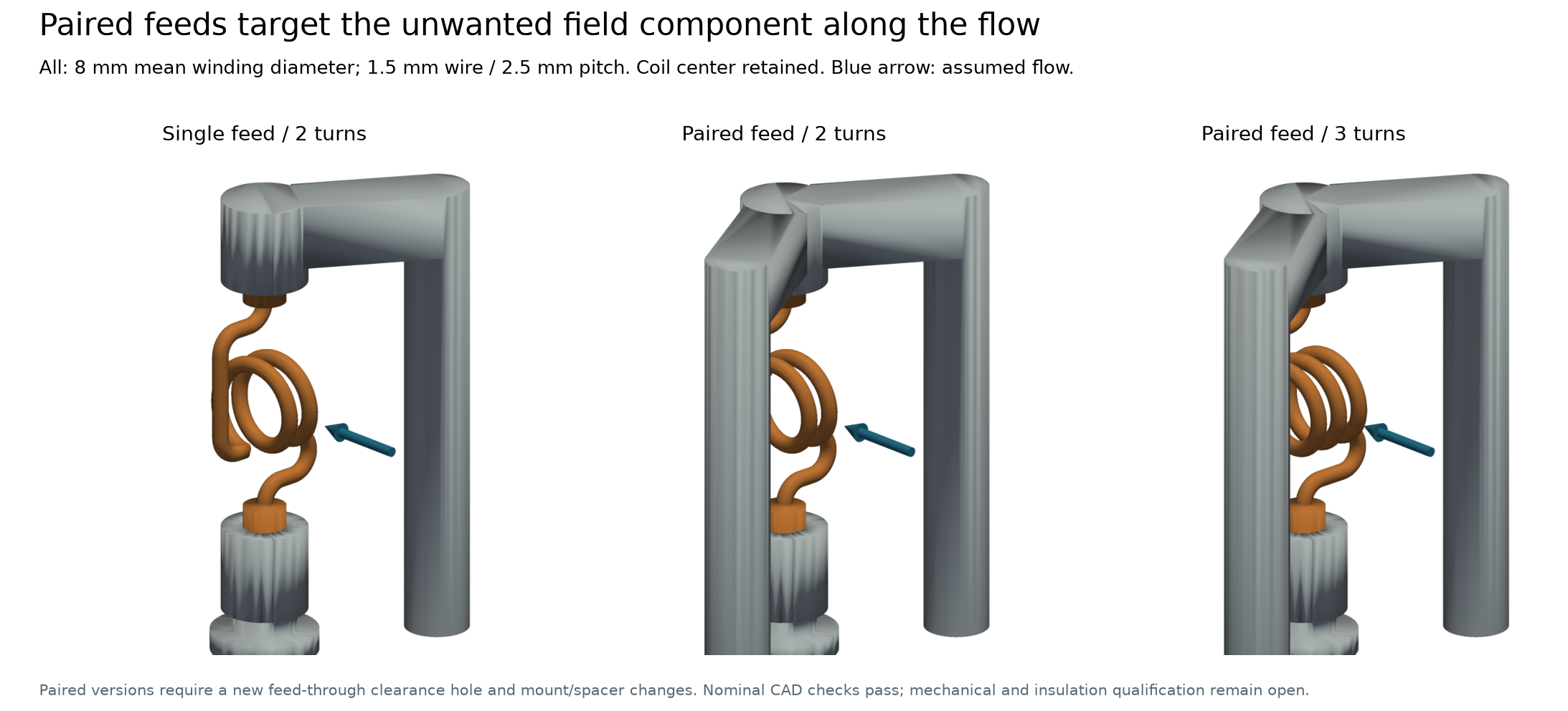
The search extended the winding comparison and then changed the feed arrangement. The selected concept has three turns, 8 mm mean diameter, 1.5 mm copper conductor and 2.5 mm pitch. A second feed/mount and a return-plate clearance hole are required; it is a fixture change. An earlier two-turn, 2 mm-conductor option preserves the original mounts and remains the simpler alternative.

A reflected feed was not accepted merely because it looked symmetric: geometry intersections had to be resolved, and the revised current division had to be solved again. Nearby feed/return currents affect both impedance and field direction. Download geometry figure.

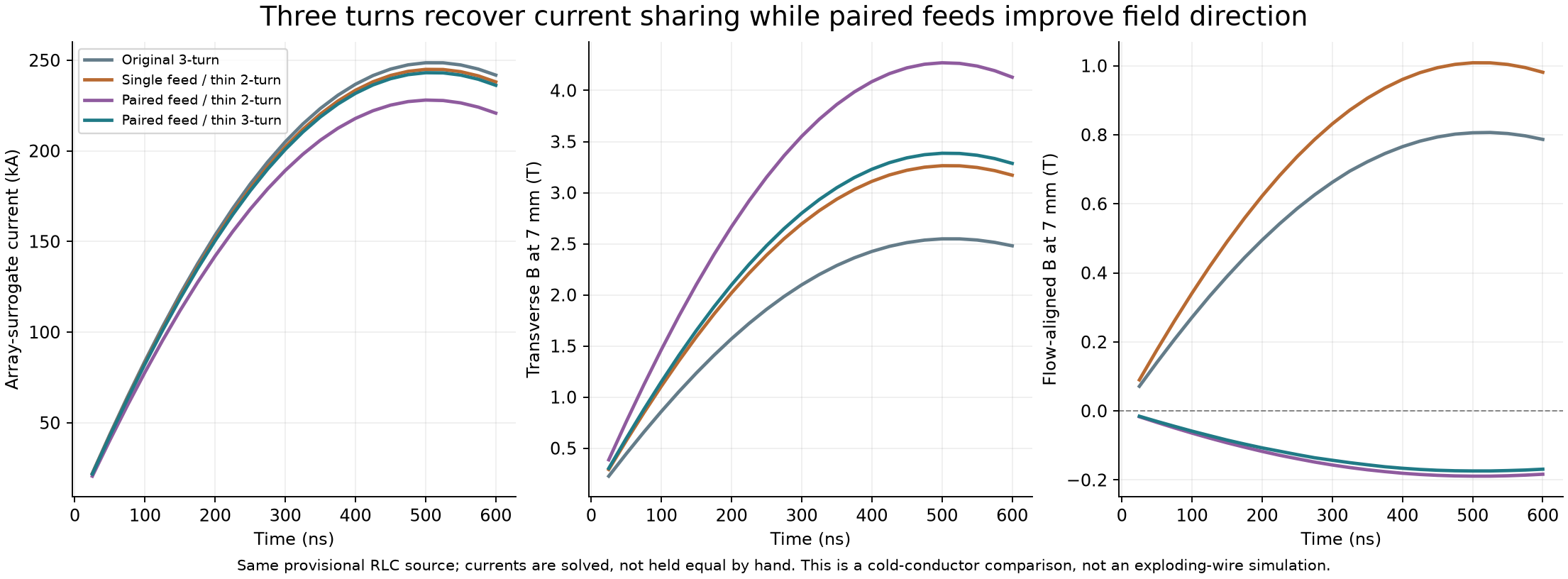
Nominal cold-conductor result	Original three-turn device	Selected paired-feed device
Maximum sampled transverse field at the upstream 7 mm probe	2.548 T	3.386 T
Maximum sampled array-branch current	248.6 kA	243.1 kA
Array-current retention	100%	97.8%
Mean frontal magnetic-pressure proxy, radius-3 mm disk at 500 ns	2.43 MPa	4.09 MPa

Matched calculations at 0.8/0.6 mm mesh targets and 25/12.5 ns timesteps retain the relative field benefit. Two levels constrain this comparison; they do not establish complete asymptotic convergence. The highest-field paired two-turn alternative retains only 91.7% of array current and misses the chosen 95% engineering target. That target is a study choice, not a universal design rule. Download circuit/field figure.

The source uses the operator-selected published Qin-1 condition, ±40 kV, 370 kA short-circuit peak and 275 ns 10–90% rise time. Qin-1 source paper. The effective 80 kV, 1.89 µF, 0.0644 Ω and 51.03 nH RLC model remains a provisional fit; the fixture is not de-embedded. The array is a fixed copper-shell surrogate. Neither real wire ablation nor coil survival is established by these cold-conductor results.

Follow the field into an actual 3D plasma calculation

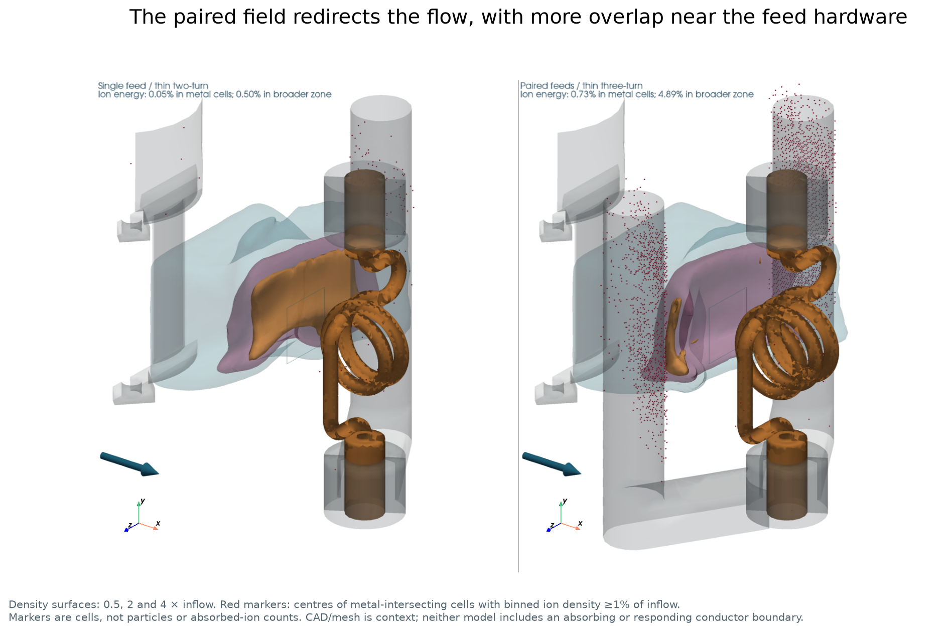
The imported field contains the entire retained coil, array and feed/return network at the 500 ns FEM state. It is held constant on a separate plasma-test clock. The assumed beam has electron density \(1.25\times10^{22}\) m⁻³, speed 100 km/s, fixed Al charge state 3.5, injected ion temperature 20 eV and isothermal electrons at 15 eV. Ion collisions and fixed resistivity are included.

At 200 ns the paired-feed field places the estimated density edge 1.34 mm farther upstream than the thin two-turn reference, or 1.76 mm relative to the original device. This edge is a falling density-profile crossing, not a verified magnetopause or bow shock. The front is still moving.

The same calculation exposes a hardware-boundary limitation: about 4.89% of ion kinetic energy lies in cells in the unqualified near-metal region, mostly near the feed assembly. The red markers identify occupied cells intersecting modeled metal, not individual impacts or absorbed particles. CAD in these views supplies spatial context; WarpX did not contain absorbing/responding conductor boundaries. Download 3D comparison.

The paired case’s mean density on the fixed readout plane is 1.29% of inflow, below its 2% numerical density floor. Its tiny flux and plane velocities are unqualified leakage metrics. The viewer marks that flux and hides the velocity. No radial wire-plume source, ablation, radiation, evolving ionization or plasma-to-circuit feedback is included. The paired geometry also needs its own numerical qualification; checks on the reference do not transfer automatically.

The numerical checks change what we can claim

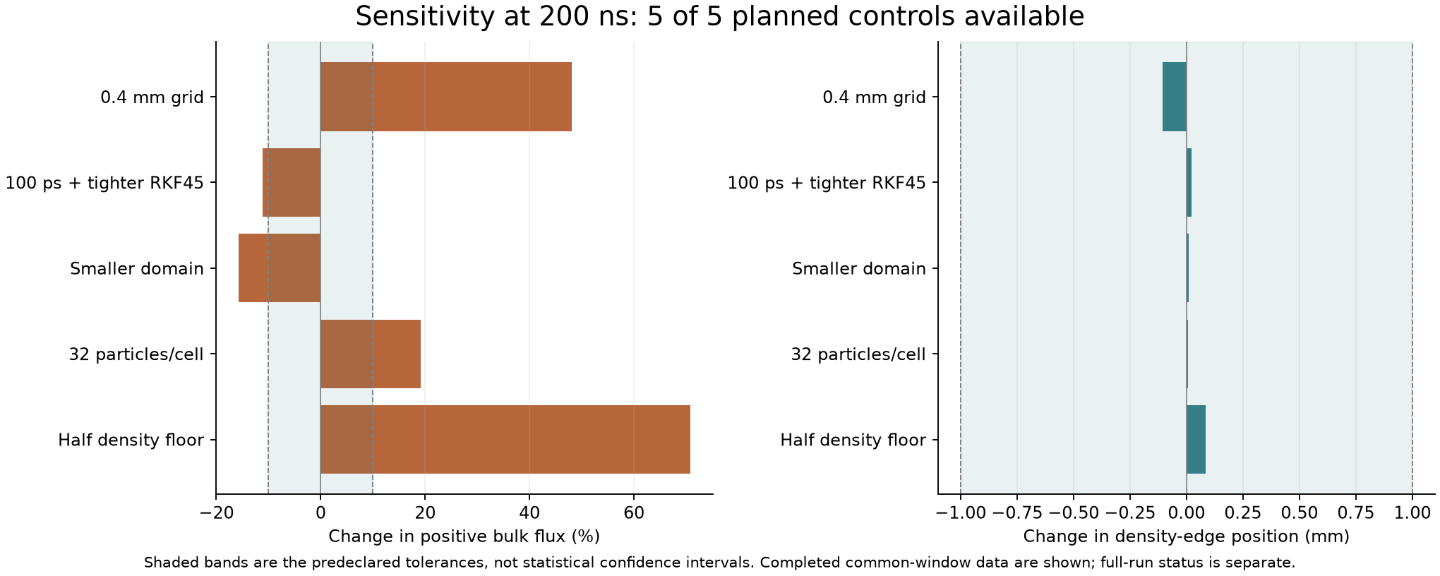
Reference control at the common 200 ns snapshot	Positive bulk-flux change	Density-edge shift
0.4 mm grid	+48.1%	−0.105 mm
100 ps timestep with tighter magnetic solver tolerance	−11.1%	+0.023 mm
Smaller domain	−15.8%	+0.008 mm
Doubled nominal particle count	+19.1%	+0.005 mm
Halved density floor	+70.8%	+0.084 mm

Zero of five meet the 10% flux tolerance; five of five meet the 1 mm edge tolerance. A stable edge does not establish converged leakage. The flux is an integral of positive cell-mean bulk flow through a fixed central plane, not a velocity-resolved one-way particle flux or global shielding efficiency. Download sensitivity figure.

The density-edge observable was added after inspecting a preliminary 140 ns state, before the sensitivity outcomes. The common 200 ns comparison was fixed before reading the original-device 200 ns result and queued control outcomes. The dated plan preserves those decisions. The finer grid also uses a slightly padded box; these are numerical-sensitivity comparisons, not isolated truncation-error estimates.

Seven of nine production runs reached 220 ns. A 90-minute limit stopped the original-device run; the host shutdown interrupted the fine-grid run. Both retain finite 200 ns outputs, with their incomplete requested durations still recorded. Recovery verified that the old processes were absent before starting untouched queued cases. Completed windows, execution success and numerical adequacy remain separate facts.

What is reusable

The general tools support user-authored geometry, mesh and Elmer models; the coil is an example, not a required schema. This study adds practical lessons for choosing model boundaries, checking a field on the receiving solver’s grid, preserving diagnostics across an interrupted campaign and exposing failed checks in the final visualization. See CAD and simulation tools.

The skill updates cover those techniques without copying the study’s dimensions, plasma assumptions or tolerances into defaults. A future measured wire-source model could use FLASH and thermodynamic/transport data, followed by a longer time-dependent interaction calculation. Those are next steps, not results of this record.

Inspect the record without rerunning the simulations

python demos/qin1_multiphysics/verify_record.py

This standard-library check verifies retained bytes, recomputes the design ratios and five sensitivity comparisons, and matches the viewer readouts to the record. It makes no model calls and launches no solver. The record guide identifies what is included and omitted. Large raw outputs, CAD, installed backends and private host paths remain outside this public excerpt; hashes identify those sources but cannot validate unavailable data.

The user supplied the experimental aim, selected source condition and overnight authorization. Early headless coil-field screening and verification ideas were contributed by @motismoore-ctrl (PR #37), motivating the full 3D CAD, coupled Elmer/circuit and plasma toolchain used here. The assistant performed the design/search, numerical work and reporting. The retained checks are not a separate independent scientific review. Software identities are frozen in study metadata: Elmer 26.2.1 with an isolated solver-core patch and native WarpX 26.09-150-g30962d771c58. This study does not change the supported dimensions or features of the packaged WarpX 26.07 PICMI capability.